4 LLM Compression Techniques That You Can’t Miss

LLMs like those from Google and OpenAI have shown incredible abilities. But their power comes at a cost. These massive models are slow, expensive to run, and difficult to deploy on everyday devices. This is where LLM compression techniques come in. These methods shrink models, making them faster and more accessible without a major loss in performance. This guide explores four key techniques: model quantization, model pruning methods, knowledge distillation in LLMs, and Low-Rank Adaptation (LoRA), complete with hands-on code examples.

Why Do We Need LLM Compression?

Before diving into the “how,” let’s understand the “why.” Compressing LLMs offers clear advantages that make them practical for real-world use.

• Reduced Model Size: Smaller models require less storage, making them easier to host and distribute.
• Faster Inference: A compact model can generate responses more quickly. This improves the user experience in applications like chatbots.
• Lower Costs: Reduced size and faster speed lead to lower needs for memory and processing power. This cuts down on cloud computing and energy costs.
• Greater Accessibility: Compression allows powerful models to run on devices with limited resources, like smartphones and laptops.

Technique 1: Quantization – Doing More with Less

Model quantization is one of the most popular and effective LLM compression techniques. It works by reducing the precision of the numbers (weights) that make up the model. Think of it like saving a high-resolution photo as a compressed JPEG; you lose a tiny amount of detail, but the file size shrinks dramatically. Most models are trained using 32-bit floating-point numbers (FP32). Quantization converts these to smaller 8-bit integers (INT8) or even 4-bit integers.

This image visually explains quantization, where continuous, high-precision FP32 (32-bit floating-point) values are mapped to a limited set of discrete, lower-precision INT4 (4-bit integer) values. Essentially, it shows how a wide range of floating-point numbers are approximated by a smaller, fixed number of integer levels to reduce memory and computation, though this can introduce some precision loss.

Hands-On: 4-bit Quantization with Hugging Face

Let’s quantize a model using the Hugging Face transformers and bitsandbytes library. This example shows how to load a model in 4-bit precision, significantly reducing its memory footprint.

Step 1: Install Libraries
First, ensure you have the necessary libraries installed.

!pip install transformers torch accelerate bitsandbytes -q

Step 2: Load and Compare Models
We will load a standard model and then its quantized version to see the difference.

import torch

from transformers import AutoModelForCausalLM, AutoTokenizer

# We use a smaller, well-known model for this demonstration

model_id = "gpt2"

print(f"Loading tokenizer for model: {model_id}")

tokenizer = AutoTokenizer.from_pretrained(model_id)

print("\n-----------------------------------")

print("Loading original model in FP32...")

# Load the original model in full precision (Float32)

model_fp32 = AutoModelForCausalLM.from_pretrained(model_id)

# Check the memory footprint of the original model

print("\nOriginal model memory footprint:")

# Calculate memory footprint manually

mem_fp32 = sum(p.numel() * p.element_size() for p in model_fp32.parameters())

print(f"{mem_fp32 / 1024**2:.2f} MB")

print("\n-----------------------------------")

print("Loading model with 4-bit quantization...")

# Load the same model with 4-bit quantization enabled

model_4bit = AutoModelForCausalLM.from_pretrained(

   model_id,

   load_in_4bit=True,

   device_map="auto" # Automatically uses the GPU if available

)

# Check the memory footprint of the 4-bit model

print("\n4-bit quantized model memory footprint:")

# Calculate memory footprint manually

mem_4bit = sum(p.numel() * p.element_size() for p in model_4bit.parameters())

print(f"{mem_4bit / 1024**2:.2f} MB")

print("\nNotice the significant reduction in memory usage!")

Output:

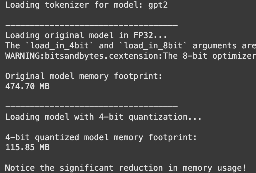
You will notice a significant reduction in the model’s memory usage with almost no change to the quality of its output for most tasks.

Technique 2: Pruning – Trimming Away Unused Connections

Model pruning methods work by removing parts of the neural network that contribute the least to its output. It’s like trimming a plant to encourage healthier growth. You can remove individual weights (unstructured pruning) or entire groups of neurons (structured pruning). While powerful, pruning can be complex to implement correctly.

Unstructured pruning, for instance, removes individual weights based on their magnitude, creating a sparse model. While this makes the model smaller, it can be difficult for hardware to take advantage of the sparse structure. Structured pruning removes entire blocks, like neurons or layers, which is often more hardware-friendly.

The image illustrates different strategies for pruning components like the Vision Transformer (ViT) and the Large Language Model (LLM) using “pruning layers” to reduce model size and improve efficiency. Specifically, (a) shows pruning in the visual encoder, (b) focuses on pruning within the LLM, and (c) introduces an “instruction-guided component” to dynamically prune visual tokens based on textual instructions, enhancing efficiency for tasks like video understanding.

Technique 3: Knowledge Distillation – The Student-Teacher Approach

Knowledge distillation in LLMs is a fascinating process. A large, highly accurate “teacher” model trains a smaller “student” model. The student learns to mimic the teacher’s thought process (its output probabilities), not just the final answer. This allows the smaller model to achieve performance far beyond what it could by training on the data alone.

This image illustrates three knowledge distillation methods in machine learning: offline, online, and self-distillation. Offline distillation uses a pre-trained “teacher” to train a “student”, while online distillation trains both simultaneously, and self-distillation involves a single model acting as both teacher and student (e.g., deeper layers teaching shallower ones). The orange “teacher” models are pre-trained, while the blue “student” models (including the combined “teacher/student” in self-distillation) are “to be trained”. 

Hands-On: Conceptual Distillation with Hugging Face

Implementing a full distillation pipeline is involved, but the core idea can be understood through the Hugging Face Trainer API.

from transformers import TrainingArguments, Trainer

# This is a conceptual example to illustrate the process.

# To run this, you would need:

# 1. A defined 'teacher_model' (a large, pre-trained model).

# 2. A defined 'student_model' (a smaller model to be trained).

# 3. A 'your_dataset' object for training.

# Define Training Arguments

training_args = TrainingArguments(

   output_dir="./student_model_distilled",

   num_train_epochs=1, # Example value

   per_device_train_batch_size=8, # Example value

   # ... other training arguments

)

# Create a custom Trainer to modify the loss function

class DistillationTrainer(Trainer):

   def compute_loss(self, model, inputs, return_outputs=False):

       # This is the core of knowledge distillation.

       # The loss function is a weighted average of two components:

       #   a) The student's standard loss on the data (e.g., Cross-Entropy).

       #   b) The distillation loss, which measures how well the student's

       #      output distribution matches the teacher's.

       # This part is conceptual and requires a full implementation.

       print("Inside custom compute_loss - this is where distillation logic would go.")

       # For example:

       # student_outputs = model(**inputs)

       # student_loss = student_outputs.loss

       # with torch.no_grad():

       #     teacher_outputs = teacher_model(**inputs)

       # distillation_loss = some_kl_divergence_loss(student_outputs.logits, teacher_outputs.logits)

       # combined_loss = 0.5 * student_loss + 0.5 * distillation_loss

       # Returning a dummy loss to prevent errors in this conceptual example

       dummy_outputs = model(**inputs)

       return (dummy_outputs.loss, dummy_outputs) if return_outputs else dummy_outputs.loss

print("The DistillationTrainer class is defined conceptually.")

print("A full implementation would require a teacher model, student model, and a dataset.")

This process effectively transfers the “knowledge” from the large model to the smaller one.

Technique 4: Low-Rank Adaptation (LoRA) – Efficient Fine-Tuning

While not a method to shrink a base model, Low-Rank Adaptation (LoRA) is a technique to compress the changes made during fine-tuning. Instead of retraining all the billions of parameters in a model, LoRA freezes the original model and injects tiny, trainable “adapter” layers. These adapters are much smaller, making the fine-tuning process faster and the resulting fine-tuned model much more memory-efficient to store and switch between.

This diagram explains LoRA (Low-Rank Adaptation) for efficient model fine-tuning: during training, a small, trainable low-rank adaptation matrix (BA) is added to the frozen pretrained weights (W). After training, this low-rank matrix is merged with the original weights, effectively creating a specialized model (W + BA) without increasing inference latency or memory footprint during deployment. This significantly reduces computational resources and storage requirements compared to full fine-tuning.

Hands-On: Fine-Tuning with LoRA and PEFT

The Hugging Face PEFT (Parameter-Efficient Fine-Tuning) library makes applying LoRA simple.

Step 1: Install Libraries

!pip install peft -q 

Step 2: Apply LoRA and Compare Parameter Counts

from peft import get_peft_model, LoraConfig, TaskType

from transformers import AutoModelForCausalLM

model_id = "gpt2"

model = AutoModelForCausalLM.from_pretrained(model_id)

# Define the LoRA configuration

lora_config = LoraConfig(

   task_type=TaskType.CAUSAL_LM, # Specify the task type

   r=8,  # Rank of the update matrices. Lower rank means fewer parameters.

   lora_alpha=32, # A scaling factor for the learned weights.

   lora_dropout=0.1, # Dropout probability for LoRA layers.

   target_modules=["c_attn"] # Apply LoRA to the attention layers of GPT-2.

)

# Wrap the base model with the LoRA adapters

lora_model = get_peft_model(model, lora_config)

print("--- Original Model ---")

# Get the total number of parameters for the original model

total_params = sum(p.numel() for p in model.parameters())

print(f"Total parameters: {total_params:,}")

print("\n--- LoRA Adapted Model ---")

# The PeftModel object has the print_trainable_parameters method

lora_model.print_trainable_parameters()

print("\nNote how LoRA reduces trainable parameters by over 99%!")

print("This makes fine-tuning much more efficient.")

Output:

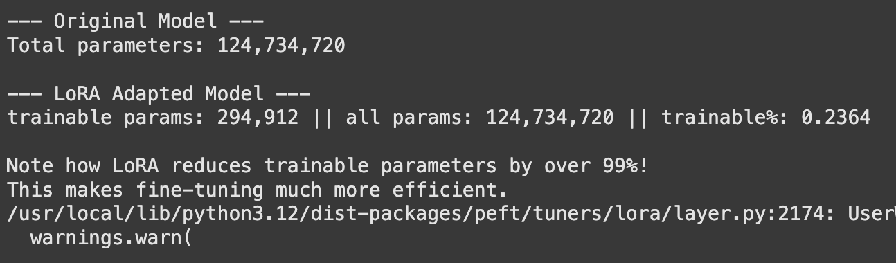
The output will show a dramatic reduction (often over 99%) in the number of parameters that need to be trained and stored. This makes it possible to fine-tune and manage many different versions of a model for various tasks without storing huge model files for each one.

You can find the full Colab notebook here: Colab

Conclusion

Large Language Models are here to stay, but their massive size presents a real challenge. LLM compression techniques are the key to unlocking their potential for a wider range of applications. Whether it’s the straightforward approach of model quantization, the surgical precision of model pruning methods, the clever mentorship of knowledge distillation in LLMs, or the efficiency of Low-Rank Adaptation (LoRA), these methods make AI more practical. The right technique depends on your specific needs, but combining them can often lead to the best results.

Frequently Asked Questions

Harsh Mishra is an AI/ML Engineer who spends more time talking to Large Language Models than actual humans. Passionate about GenAI, NLP, and making machines smarter (so they don’t replace him just yet). When not optimizing models, he’s probably optimizing his coffee intake. 🚀☕